Coding a perceptron from scratch in C++

View project on GitHub

What is a perceptron?

In very simple terms, a perceptron is a binary classifier that takes a vector input and outputs a 0 or a 1.

How does a perceptron work?

A perceptron has 2 tunable parameters:

• A vector of weights
• A bias

Given an input (assuming the input shape matches the shape of the perceptron’s weights), classification is performed as follows:

1. Calculate the dot product of the perceptron’s weights and the input vector.
2. Add the perceptron’s bias to the dot product.

Finally, classify the point as 1 if the total sum is positive. Otherwise, classify it as a 0.

Initialization

Before a perceptron is “trained” to classify your data well, it must first be given some set of weights and some bias. During the learning process (below), these weights and this bias will be altered.

Given enough time and a linearly separable (!) dataset, a perceptron will always converge, no matter what its starting weights were. In this program, we’ll initialize weights to {1, 1, ...} and bias to 0.

Learning process

Learning consists of repeating an identical process a total of n times where n is the number of epochs. Learning also requires a learning rate, lr, which specifies how sloppily-but-quickly or carefully-but-slowly our perceptron arrives at an ideal weights and bias.

At each epoch, the following adjustments are made for each sample (simplified):

1. If the sample is currently being classified correctly, change no weights.
2. Otherwise,
   • If the sample is of type 0 but is being classified 1, increase the weights.
   • If the sample is of type 1 but is being classified 0, decrease the weights.

Example usage

First, the program asks us how many samples (points) we would like to define, as well as their dimensionality. To make this example easy to visualize, let’s use 2-dimensional points.

How many samples? 6
How many dimensions? 2

The program then asks for the locations of our points. Let’s use these as our samples: 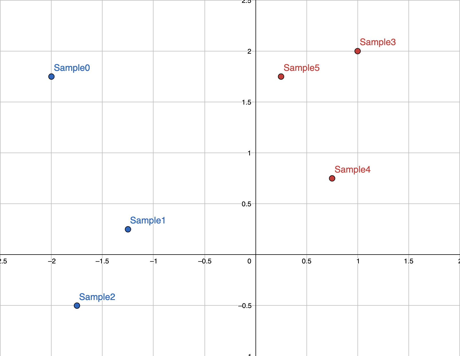Note, x_0 corresponds to the x-axis, x_1 corresponds to the y-axis.

The program also needs to know if the sample is blue or red. Let’s set the is_type_A value of a sample to 1 if it’s blue, otherwise 0 (meaning red).

Sample 0
x_0? -2
x_1? 1.75
is_type_A? 1
...
Sample 5
x_0? 0.25
x_1? 1.75
is_type_A? 0

At this point, the perceptron is ready to train. The program asks for a learning rate and a number of epochs. (Refer to How does a perceptron work? above.)

What is the learning rate? 0.1
How many epochs? 200

That’s it! The perceptron quickly trains on the small dataset. The program displays the parameters of the perceptron before and after training.

Before training: Perceptron(weights: {1.00, 1.00}, bias: 0.00, lr: 0.10)
>After training: Perceptron(weights: {-0.30, 0.02}, bias: -0.20, lr: 0.10)

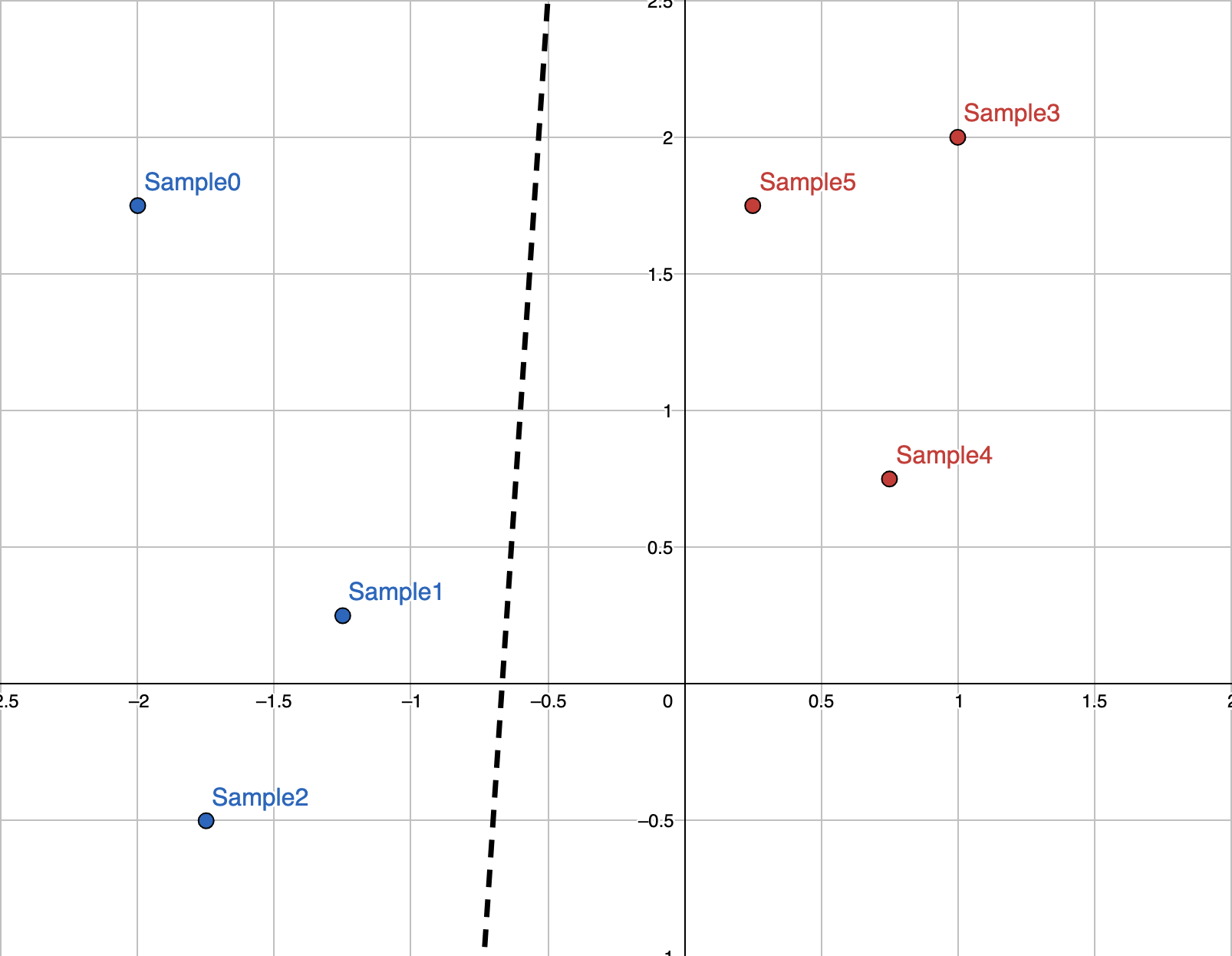
Using the tuned parameters we can plot the line that our perceptron has created to separate the data. Recall that a weights of {-0.3, 0.02} and a bias of -0.2 means the perceptron classifies a given point $(a, b)$ based on $-0.3a + 0.02b - 0.2 > 0$.

We can generalize this to x and y, giving us the inequality for a line. All points above the line will be classified as blue, and those below it will be classified as red. As you can see, the parameters of the trained perceptron have created a very good separating line for the data:

Finally, the program shows how much of the training data is now successfully classified by the perceptron.

Predicted 1 for Sample({-2.00, 1.75}, is_type_A: 1) ✓
Predicted 1 for Sample({-1.25, 0.25}, is_type_A: 1) ✓
Predicted 1 for Sample({-1.75, -0.50}, is_type_A: 1) ✓
Predicted 0 for Sample({1.00, 2.00}, is_type_A: 0) ✓
Predicted 0 for Sample({0.75, 0.75}, is_type_A: 0) ✓
Predicted 0 for Sample({0.25, 1.75}, is_type_A: 0) ✓